In this tutorial, we are going to see how we can create a simple drop down list in Excel.
Video (How to create drop down list in Excel)
If you would like to be notified of these videos, please subscribe to our YouTube channel.
What are drop down lists?
A drop down list is a way to implement data validation and improve data entry in Excel.
- Optionally, you can provide message to guide the user on data entry.
- It informs the user what values are allowed
- It allows the user to choose from a list instead of typing the value.
- It limits what values can be entered in a cell.
- Optionally, you can provide an error message when the user does not enter a valid value.
Can we see an example?
Let’s take a simple example.
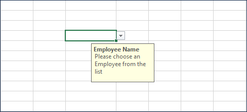
In the image above, you can see the message for the user instructing what data is expected in that cell.
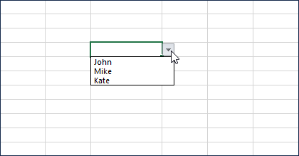
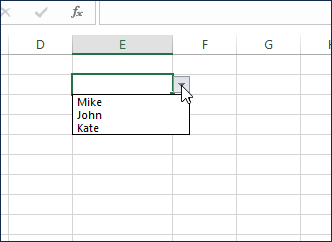
When click on the downward arrow button, we see John, Mike, and Kate. John, Mike and Kate are the allowed values
User can choose Mike from the list instead of typing the value.
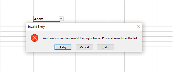
If the user enters a value not in the list, it will not allow. If the user enters an invalid value, there will be an error message.
Now, we know what a drop down list is, let’s see how we can build this.
How to build a drop down list?
Step 1: Enter list of values
In a blank new sheet, let’s type the following information.
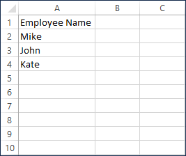
First value (Employee Name) refers to the header or field name. Then, we have entered names of three employees.
Step 2: Convert the data to a table
Select all four cells with data and press Ctrl+T
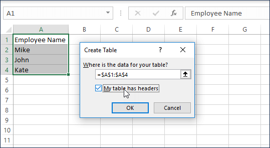
Please make sure that you check the box ‘My Table has headers’.
Once you hit OK, you will see that the table is created.
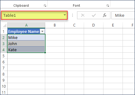
The Name Box will display Table1. That is the name of our Table.
Step 3: Create a name to our list
Select the list of values and then press Ctrl+F3 to open Name Manager. Or select from the Formulas ribbon as shown below.
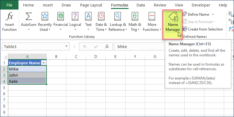
In the following window, click on New, as we are creating a new Name.
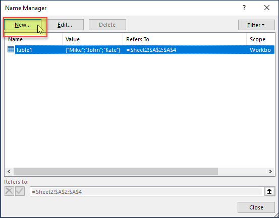
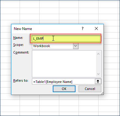
In the next window that opens, specify the name we want to give. I usually provide all my lists names that start with L. For example, L_EMP as this is a list of Employee Names.
Step 4: Implement Data validation
We will implement first in a single cell.
Let’s select the cell where we want to apply data validation or drop down list. I am choosing cell E2.
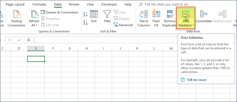
Then select Data Validation from the Data ribbon.
In the following window, choose List for the ‘Allow:’
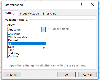
Note: There are different types of data validation that can be done in Excel. We are currently focusing on a simple drop down list of names. Hence, we are choosing ‘List’.
Then, we need to inform Excel where the List is.
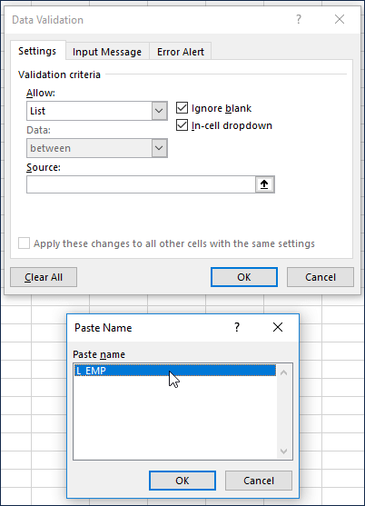
Click inside the Source field. Press F3.
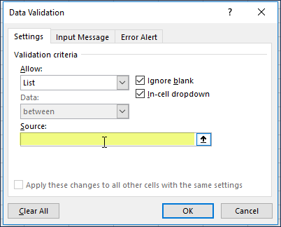
Choose our name L_EMP and press OK.
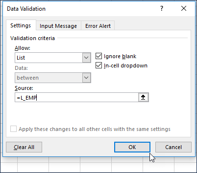
You will now see that the Source is L_EMP (our list of employee names). Press OK in the dialog box.
That’s it. Now, we have implemented the drop down list in cell E2.
Optional:
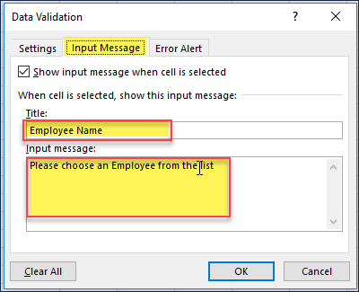
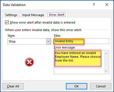
A couple of optional steps are to provide the input message and error alert message. These are recommended if the user who is going to use the file is not familiar with the data and needs direction.
Extensions
So far, we have learnt how to implement drop-down list in one cell. Let’s look at a couple of ways to extend this technique further.
More than one cell especially when cells are far apart
You can copy this cell (which has the drop down list) and paste in another cell. The data validation and drop down list will also be copied over. So, if you need the same drop down in different cells (far apart), it is easy. Just copy and paste.
Inside Tables
In almost all my templates, I use drop down lists inside tables. For example, we have an Applications table where we must select the Job ID from list of available Job IDs (coming from another sheet). This means that the drop-down list should be enabled for each application. Fortunately, Excel makes it easy. We can follow similar steps as outlined earlier.
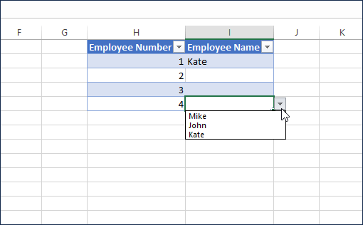
Let’s say we have a table (call it DATA table) as shown below with just two columns. Employee Number and Employee Name. We want to implement drop down list for Employee Name column.
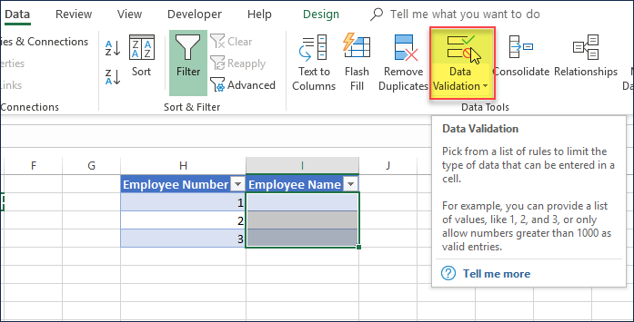
Select the three cells in Employee Name column.
Then, follow steps as mentioned earlier to choose L_EMP as source of our data validation list.
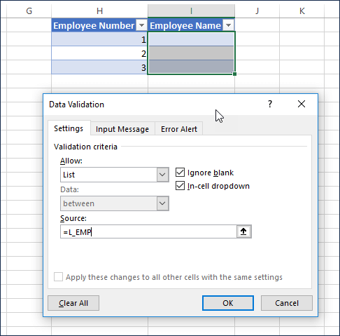
That’s it.
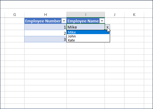
The amazing part of this method is that 1) the list of values can grow over time and 2) the data table cells can also be extended without any issues.
If we enter a fourth row in the DATA table. Type 4 in Employee Number and see that the Employee Name column will have a drop down for the fourth row as well automatically.
Note of Caution
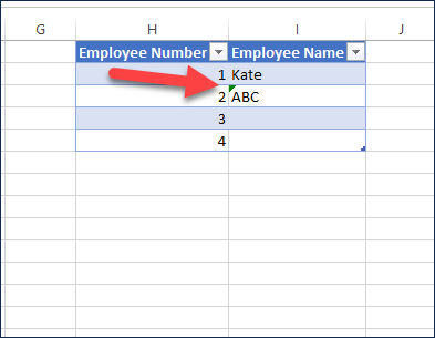
Drop down lists are not perfect when it comes to data validation. There are ways invalid values might get into the cells. An error icon will appear in such cases.
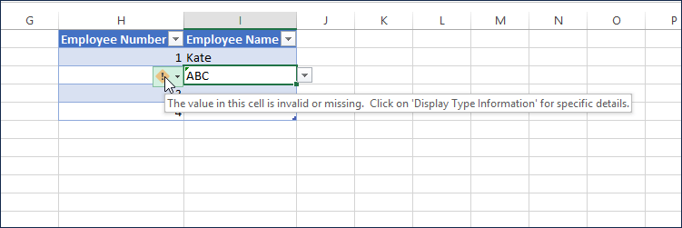
When you click on the cell, you will see the following message.
A couple of reasons for this to happen
- If we copy (from somewhere) and paste values in the cell, they don’t return errors and Excel allows the invalid values.
- After we implement the drop down list and have entered some values in our DATA table, if we change our List of Values, DATA Table will not update automatically.
Please take care and ensure that the above two scenarios do not happen with your file. If it happens, please fix the data entry and update the cell value to a valid one from the list.
Adding drop-down lists enhances the user experience in Excel templates and I use this technique in all my templates. I hope this tutorial is useful to you.
