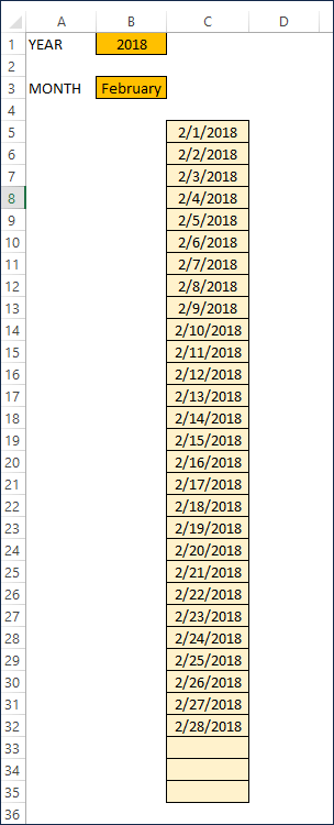
In this tutorial, we will learn how to calculate dates of any chosen month. If we enter Year and Month, we want to automatically calculate the dates of the specific month, as shown below.
If you prefer video demo, please watch this.
Subscribe to our YouTube Channel
First, let’s set up our data input. We will let the user select Year and Month as two inputs.
STEP 1: Set up Year Input
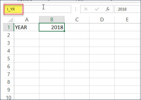
Type YEAR in cell A1
Type 2018 in cell B1.
With cell B1 selected, type I_YR in Namebox.
STEP 2: Set up Month Input
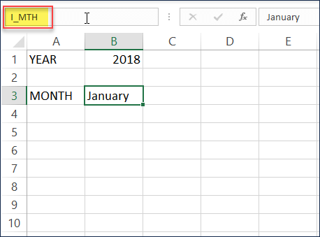
Type MONTH in cell A3
Type January in cell B3.
With cell B3 selected, type I_MTH in Namebox.
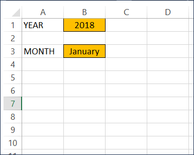
Let’s fill the two input cells to a different color and apply borders so that it is clearly visible as input cells.
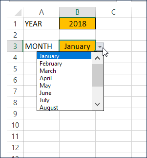
STEP 3: Implement Drop down list for Month input
We want the Month input to have data validation and a drop down list that shows all the months. To do this, we need a list of Month names.
Let’s create a new sheet. Type January in a cell. Then click on the cell and find the bottom right corner with your mouse and drag down to auto-fill all the 12 months.
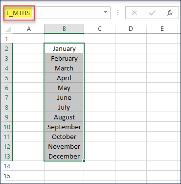
Now, select the 12 months and name this list L_MTHS (as it is a list).
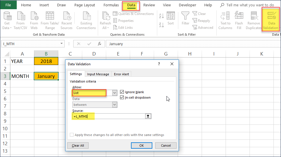
Let’s go back to Sheet 1 and apply data validation to the Month Input cell I_MTH as shown below.
In the previous video, we explained how to create such a drop down list.
STEP 4: Formula to create the starting date for our calendar
Go to cell C5 and type the formula
=DATE(I_YR,MATCH(I_MTH,L_MTHS,0),1)
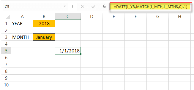
DATE function needs YEAR, MONTH, DAY as parameters. We get YEAR value from I_YR cell.
For Month, Excel needs the month number such as 1, 2 and not a text string such as January, February. To convert user’s input of January to 1 and February to 2, we use the MATCH function.
MATCH function takes the input Month I_MTH and searches in the L_MTHS list and returns the row number where it found.
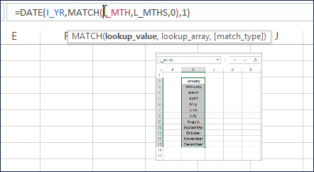
Since January will be found in the first row of the L_MTHS list, it will return 1 as the result.
STEP 5: Formula to create the other dates for our calendar
In cell C6, we need to use a formula to calculate the second date of the month we chose. Excel treats dates as numbers and hence to find the second date, we can just type = C5+1
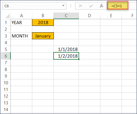
That would calculate the second day.
Extend the formula down to reach the 31st day.
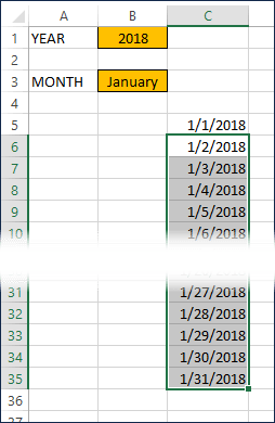
Now, if you change the Year to 2017, the dates would show for 2017 January.
If you choose 2018 as Year and February as Month, then we will see the below.
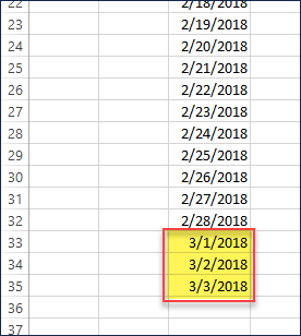
If our goal is to display only dates in February, this is not ideal, as it shows the first 3 days of March. This is because, we are just calculating 31 days and since February has only 28 days, the next 3 days are from March.
If we choose April the last day will show as May 1st, as April has only 30 days.
We will solve this problem by adding logic to our formula. There are many ways to do this. We will use one of the methods.
First, the logic we need to implement is
IF Date > End of Month, then do not display date. Otherwise display date.
In Excel, we can implement as
=IFERROR(IF(C5+1>EOMONTH($C$5,0),””,C5+1),””)
EOMONTH function is taking the first date (C5) of our month and finds the end of the same month (as we use 0 as the second parameter)
If we use 1 as the second parameter, then it will calculate the end of next month. If we use -1, it will calculate end of previous month.
You would also notice that I am using the $C$5 instead of C5. This $ symbol locks the column and row when we drag the formula to the cells below. This is called absolute cell reference. Explained in the video https://youtu.be/bTI_GIpw8fU
In this scenario, your result will be the same even if we used C5 instead of $C$5.
IFERROR is used to display nothing when an invalid value appears.
That’s it. With just two formulas, we have now created a way to calculate and display dates of any month chosen.
Note:
In this tutorial, we have used two formulas to calculate dates. 1 for the first date of the month and 1 for all the other dates. I usually try to avoid this when I build templates. If we had one formula for all the dates, it will be easier for maintenance, as I would have to make changes to only one and also it will be easy to remember. However, making it into one formula will make the formula more advanced and hence we will leave it to a future video.
Functions Used: DATE, IFERROR, EOMONTH, IF, MATCH
Features Used: Named Range, Data Validation, Drop-down list, Cell References, Formulas